
Original: https://towardsdatascience.com/types-of-convolutions-in-deep-learning-717013397f4d
Let me give you a quick overview of different types of convolutions and what their benefits are. For the sake of simplicity, I’m focussing on 2D convolutions only.
First we need to agree on a few parameters that define a convolutional layer.
(a.k.a. atrous convolutions)
Dilated convolutions introduce another parameter to convolutional layers called the dilation rate. This defines a spacing between the values in a kernel. A 3×3 kernel with a dilation rate of 2 will have the same field of view as a 5×5 kernel, while only using 9 parameters. Imagine taking a 5×5 kernel and deleting every second column and row.
This delivers a wider field of view at the same computational cost. Dilated convolutions are particularly popular in the field of real-time segmentation. Use them if you need a wide field of view and cannot afford multiple convolutions or larger kernels.
(a.k.a. deconvolutions or fractionally strided convolutions)
Some sources use the name deconvolution, which is inappropriate because it’s not a deconvolution. To make things worse deconvolutions do exists, but they’re not common in the field of deep learning. An actual deconvolution reverts the process of a convolution. Imagine inputting an image into a single convolutional layer. Now take the output, throw it into a black box and out comes your original image again. This black box does a deconvolution. It is the mathematical inverse of what a convolutional layer does.
A transposed convolution is somewhat similar because it produces the same spatial resolution a hypothetical deconvolutional layer would. However, the actual mathematical operation that’s being performed on the values is different. A transposed convolutional layer carries out a regular convolution but reverts its spatial transformation.
At this point you should be pretty confused, so let’s look at a concrete example. An image of 5×5 is fed into a convolutional layer. The stride is set to 2, the padding is deactivated and the kernel is 3×3. This results in a 2×2 image.
If we wanted to reverse this process, we’d need the inverse mathematical operation so that 9 values are generated from each pixel we input. Afterward, we traverse the output image with a stride of 2. This would be a deconvolution.
A transposed convolution does not do that. The only thing in common is it guarantees that the output will be a 5×5 image as well, while still performing a normal convolution operation. To achieve this, we need to perform some fancy padding on the input.
As you can imagine now, this step will not reverse the process from above. At least not concerning the numeric values.
It merely reconstructs the spatial resolution from before and performs a convolution. This may not be the mathematical inverse, but for Encoder-Decoder architectures, it’s still very helpful. This way we can combine the upscaling of an image with a convolution, instead of doing two separate processes.
In a separable convolution, we can split the kernel operation into multiple steps. Let’s express a convolution as y = conv(x, k) where y is the output image, x is the input image, and k is the kernel. Easy. Next, let’s assume k can be calculated by: k = k1.dot(k2). This would make it a separable convolution because instead of doing a 2D convolution with k, we could get to the same result by doing 2 1D convolutions with k1 and k2.
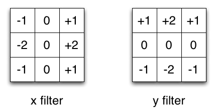
Take the Sobel kernel for example, which is often used in image processing. You could get the same kernel by multiplying the vector [1, 0, -1] and [1,2,1].T. This would require 6 instead of 9 parameters while doing the same operation. The example above shows what’s called a spatial separable convolution, which to my knowledge isn’t used in deep learning.
Edit: Actually, one can create something very similar to a spatial separable convolution by stacking a 1xN and a Nx1 kernel layer. This was recently used in an architecture called EffNet showing promising results.
In neural networks, we commonly use something called a depthwise separable convolution. This will perform a spatial convolution while keeping the channels separate and then follow with a depthwise convolution. In my opinion, it can be best understood with an example.
Let’s say we have a 3×3 convolutional layer on 16 input channels and 32 output channels. What happens in detail is that every of the 16 channels is traversed by 32 3×3 kernels resulting in 512 (16×32) feature maps. Next, we merge 1 feature map out of every input channel by adding them up. Since we can do that 32 times, we get the 32 output channels we wanted.
For a depthwise separable convolution on the same example, we traverse the 16 channels with 1 3×3 kernel each, giving us 16 feature maps. Now, before merging anything, we traverse these 16 feature maps with 32 1×1 convolutions each and only then start to them add together. This results in 656 (16x3x3 + 16x32x1x1) parameters opposed to the 4608 (16x32x3x3) parameters from above.
The example is a specific implementation of a depthwise separable convolution where the so called depth multiplier is 1. This is by far the most common setup for such layers.
We do this because of the hypothesis that spatial and depthwise information can be decoupled. Looking at the performance of the Xception model this theory seems to work. Depthwise separable convolutions are also used for mobile devices because of their efficient use of parameters.
This concludes our little tour through different types of convolutions. I hope it helped to get a brief overview of the matter. Drop a comment if you have any remaining questions and check out this GitHub page for more convolution animations.
Source:
https://towardsdatascience.com/types-of-convolutions-in-deep-learning-717013397f4d
Semantic segmentation is understanding an image at pixel level i.e, we want to assign each pixel in the image an object class. For example, check out the following images.


Left: Input image. Right: It’s semantic segmentation. Source.
Apart from recognizing the bike and the person riding it, we also have to delineate the boundaries of each object. Therefore, unlike classification, we need dense pixel-wise predictions from our models.
VOC2012 and MSCOCO are the most important datasets for semantic segmentation.
Before deep learning took over computer vision, people used approaches like TextonForest and Random Forest based classifiers for semantic segmentation. As with image classification, convolutional neural networks (CNN) have had enormous success on segmentation problems.
One of the popular initial deep learning approaches was patch classification where each pixel was separately classified into classes using a patch of image around it. Main reason to use patches was that classification networks usually have full connected layers and therefore required fixed size images.
In 2014, Fully Convolutional Networks (FCN) by Long et al. from Berkeley, popularized CNN architectures for dense predictions without any fully connected layers. This allowed segmentation maps to be generated for image of any size and was also much faster compared to the patch classification approach. Almost all the subsequent state of the art approaches on semantic segmentation adopted this paradigm.
Apart from fully connected layers, one of the main problems with using CNNs for segmentation is pooling layers. Pooling layers increase the field of view and are able to aggregate the context while discarding the ‘where’ information. However, semantic segmentation requires the exact alignment of class maps and thus, needs the ‘where’ information to be preserved. Two different classes of architectures evolved in the literature to tackle this issue.
First one is encoder-decoder architecture. Encoder gradually reduces the spatial dimension with pooling layers and decoder gradually recovers the object details and spatial dimension. There are usually shortcut connections from encoder to decoder to help decoder recover the object details better. U-Net is a popular architecture from this class.

U-Net: An encoder-decoder architecture. Source.
Architectures in the second class use what are called as dilated/atrous convolutionsand do away with pooling layers.

Dilated/atrous convolutions. rate=1 is same as normal convolutions. Source.
Conditional Random Field (CRF) postprocessing are usually used to improve the segmentation. CRFs are graphical models which ‘smooth’ segmentation based on the underlying image intensities. They work based on the observation that similar intensity pixels tend to be labeled as the same class. CRFs can boost scores by 1-2%.

CRF illustration. (b) Unary classifiers is the segmentation input to the CRF. (c, d, e) are variants of CRF with (e) being the widely used one. Source.
In the next section, I’ll summarize a few papers that represent the evolution of segmentation architectures starting from FCN. All these architectures are benchmarked on VOC2012 evaluation server.
Following papers are summarized (in chronological order):
For each of these papers, I list down their key contributions and explain them. I also show their benchmark scores (mean IOU) on VOC2012 test dataset.
Key Contributions:
Explanation:
Key observation is that fully connected layers in classification networks can be viewed as convolutions with kernels that cover their entire input regions. This is equivalent to evaluating the original classification network on overlapping input patches but is much more efficient because computation is shared over the overlapping regions of patches. Although this observation is not unique to this paper (see overfeat, this post), it improved the state of the art on VOC2012 significantly.

Fully connected layers as a convolution. Source.
After convolutionalizing fully connected layers in a imagenet pretrained network like VGG, feature maps still need to be upsampled because of pooling operations in CNNs. Instead of using simple bilinear interpolation, deconvolutional layers can learn the interpolation. This layer is also known as upconvolution, full convolution, transposed convolution or fractionally-strided convolution.
However, upsampling (even with deconvolutional layers) produces coarse segmentation maps because of loss of information during pooling. Therefore, shortcut/skip connections are introduced from higher resolution feature maps.
Benchmarks (VOC2012):
| Score | Comment | Source |
|---|---|---|
| 62.2 | – | leaderboard |
| 67.2 | More momentum. Not described in paper | leaderboard |
My Comments:
Key Contributions:
Explanation:
FCN, despite upconvolutional layers and a few shortcut connections produces coarse segmentation maps. Therefore, more shortcut connections are introduced. However, instead of copying the encoder features as in FCN, indices from maxpooling are copied. This makes SegNet more memory efficient than FCN.

Segnet Architecture. Source.
Benchmarks (VOC2012):
| Score | Comment | Source |
|---|---|---|
| 59.9 | – | leaderboard |
My comments:
Key Contributions:
Explanation:
Pooling helps in classification networks because receptive field increases. But this is not the best thing to do for segmentation because pooling decreases the resolution. Therefore, authors use dilated convolution layer which works like this:

Dilated/Atrous Convolutions. Source
Dilated convolutional layer (also called as atrous convolution in DeepLab) allows for exponential increase in field of view without decrease of spatial dimensions.
Last two pooling layers from pretrained classification network (here, VGG) are removed and subsequent convolutional layers are replaced with dilated convolutions. In particular, convolutions between the pool-3 and pool-4 have dilation 2 and convolutions after pool-4 have dilation 4. With this module (called frontend module in the paper), dense predictions are obtained without any increase in number of parameters.
A module (called context module in the paper) is trained separately with the outputs of frontend module as inputs. This module is a cascade of dilated convolutions of different dilations so that multi scale context is aggregated and predictions from frontend are improved.
Benchmarks (VOC2012):
| Score | Comment | Source |
|---|---|---|
| 71.3 | frontend | reported in the paper |
| 73.5 | frontend + context | reported in the paper |
| 74.7 | frontend + context + CRF | reported in the paper |
| 75.3 | frontend + context + CRF-RNN | reported in the paper |
My comments:
Key Contributions:
Explanation:
Atrous/Dilated convolutions increase the field of view without increasing the number of parameters. Net is modified like in dilated convolutions paper.
Multiscale processing is achieved either by passing multiple rescaled versions of original images to parallel CNN branches (Image pyramid) and/or by using multiple parallel atrous convolutional layers with different sampling rates (ASPP).
Structured prediction is done by fully connected CRF. CRF is trained/tuned separately as a post processing step.

DeepLab2 Pipeline. Source.
Benchmarks (VOC2012):
| Score | Comment | Source |
|---|---|---|
| 79.7 | ResNet-101 + atrous Convolutions + ASPP + CRF | leaderboard |
Key Contributions:
Explanation:
Approach of using dilated/atrous convolutions are not without downsides. Dilated convolutions are computationally expensive and take a lot of memory because they have to be applied on large number of high resolution feature maps. This hampers the computation of high-res predictions. DeepLab’s predictions, for example are 1/8th the size of original input.
So, the paper proposes to use encoder-decoder architecture. Encoder part is ResNet-101 blocks. Decoder has RefineNet blocks which concatenate/fuse high resolution features from encoder and low resolution features from previous RefineNet block.

RefineNet Architecture. Source.
Each RefineNet block has a component to fuse the multi resolution features by upsampling the lower resolution features and a component to capture context based on repeated 5 x 5 stride 1 pool layers. Each of these components employ the residual connection design following the identity map mindset.

RefineNet Block. Source.
Benchmarks (VOC2012):
| Score | Comment | Source |
|---|---|---|
| 84.2 | Uses CRF, Multiscale inputs, COCO pretraining | leaderboard |
Key Contributions:
Explanation:
Global scene categories matter because it provides clues on the distribution of the segmentation classes. Pyramid pooling module captures this information by applying large kernel pooling layers.
Dilated convolutions are used as in dilated convolutions paper to modify Resnet and a pyramid pooling module is added to it. This module concatenates the feature maps from ResNet with upsampled output of parallel pooling layers with kernels covering whole, half of and small portions of image.
An auxiliary loss, additional to the loss on main branch, is applied after the fourth stage of ResNet (i.e input to pyramid pooling module). This idea was also called as intermediate supervision elsewhere.

PSPNet Architecture. Source.
Benchmarks (VOC2012):
| Score | Comment | Source |
|---|---|---|
| 85.4 | MSCOCO pretraining, multi scale input, no CRF | leaderboard |
| 82.6 | no MSCOCO pretraining, multi scale input, no CRF | reported in the paper |
Key Contributions:
Explanation:
Semantic segmentation requires both segmentation and classification of the segmented objects. Since fully connected layers cannot be present in a segmentation architecture, convolutions with very large kernels are adopted instead.
Another reason to adopt large kernels is that although deeper networks like ResNet have very large receptive field, studies show that the network tends to gather information from a much smaller region (valid receptive filed).
Larger kernels are computationally expensive and have a lot of parameters. Therefore, k x k convolution is approximated with sum of 1 x k + k x 1 and k x 1 and 1 x k convolutions. This module is called as Global Convolutional Network (GCN) in the paper.
Coming to architecture, ResNet(without any dilated convolutions) forms encoder part of the architecture while GCNs and deconvolutions form decoder. A simple residual block called Boundary Refinement (BR) is also used.

GCN Architecture. Source.
Benchmarks (VOC2012):
| Score | Comment | Source |
|---|---|---|
| 82.2 | – | reported in the paper |
| 83.6 | Improved training, not described in the paper | leaderboard |
Key Contributions:
Explanation:
ResNet model is modified to use dilated/atrous convolutions as in DeepLabv2 and dilated convolutions. Improved ASPP involves concatenation of image-level features, a 1×1 convolution and three 3×3 atrous convolutions with different rates. Batch normalization is used after each of the parallel convolutional layers.
Cascaded module is a resnet block except that component convolution layers are made atrous with different rates. This module is similar to context module used in dilated convolutions paper but this is applied directly on intermediate feature maps instead of belief maps (belief maps are final CNN feature maps with channels equal to number of classes).
Both the proposed models are evaluated independently and attempt to combine the both did not improve the performance. Both of them performed very similarly on val set with ASPP performing slightly better. CRF is not used.
Both these models outperform the best model from DeepLabv2. Authors note that the improvement comes from the batch normalization and better way to encode multi scale context.

DeepLabv3 ASPP (used for submission). Source.
Benchmarks (VOC2012):
| Score | Comment | Source |
|---|---|---|
| 85.7 | used ASPP (no cascaded modules) | leaderboard |
Source from:
Chinese Version is here:

